
Homogeneous vectors
NOTE: updated on December 28, 2023 (fixed some mistakes)
Homogeneous coordinates is an extremely useful system of coordinates origination from the field of projective geometry, and widely used in computer vision and robotics. They allow to represent certain classes of non-linear transformations in linear form, which opens up for some elegant closed-form solutions to various problems. In this blog post I am going to briefly intoroduce the idea and show how homogeneous vectors can be applied for the tasks of finding intersection of two lines at a point and finding a line through two points. This is also my first attempt of preparing a blog post as a Jupyter notebook, which is further converted into Markdown to be a part of a Hugo site.
Let’s first import NumPy and Matplotlib.
import numpy as np
from matplotlib import pyplot as plt
In simple terms, a homogeneous vector $\mathbf{x}_h \in \mathbb{P}^n$ ($\mathbb{P}^n$ means a projective space of dimension $n$) is constructed from an Euclidean vector $\mathbf{x} \in \mathbb{R}^n$ by adding one more element to the vector with value 1. An example in $\mathbb{R}^2$ can be the following:
$$ \mathbf{x} = \begin{bmatrix} 4\cr -2 \end{bmatrix} $$
$$ \mathbf{x}_h = \begin{bmatrix} 4\cr -2\cr 1 \end{bmatrix} $$
Although $\mathbf{x}_h$ here has 3 elements, we still refer to it as a member of the projective space of dimension 2, namely $\mathbb{P}^2$.
Let’s create a function e2h (for “Euclidean-to-homogeneous”) and use with the same values as in the example above:
def e2h(x):
    n = len(x)
    result = np.ones(n + 1, dtype=x.dtype)
    result[:n] = x
    return result
x = np.array([4, -2])
print(f'x = {x}')

x_h = e2h(x)
print(f'x_h = {x_h}')
x = [ 4 -2]
x_h = [ 4 -2  1]
A special feature of homogeneus vectors is that they are equivalent when scaled. So if we multiply $\mathbf{x}_h$ with, say, 7.5, it will represent the same vector, although with different values:
x_h_equivalent = x_h * 7.5

print(x_h_equivalent)
[ 30. -15. 7.5]
We can convert a homogeneous vector back to the Eucliden space by dividing all if its elements but last by the last element:
def h2e(x):
    return x[:-1] / x[-1]
Let’s see it in action:
for hvec in (x_h, x_h_equivalent):
    print('Homogeneous:', hvec)
    print('Euclidean:  ', h2e(hvec))
    print()
Homogeneous: [ 4 -2  1]
Euclidean:   [ 4. -2.]

Homogeneous: [ 30.  -15.    7.5]
Euclidean:   [ 4. -2.]
As you can see, the two equiavent homegeneous vectors got converted to the same Euclidean vector.
Let’s now take a look at a particularly useful application where homogeneous vectors come in handy, namely the task of finding an intersection of two lines and its “dual”, finding a line passing throught two points.
Points can be very naturally represented as homogeneous vectors: you just “append” 1, as in the example above. When it comes to lines, they can be represented as homogeneous vectors when we consider the following form of the line equation:
$$ a_0 x_0 + a_1 x_1 + … + a_{n-1} x_{n-1} + a_n = 0 $$
Or, for 2D plane ($\mathbb{R}^2$):
$$ a x + b y + c = 0 $$
The coefficients in this form of the line equation constitute the element of the homegeneous vector. For out 2D-case, this simply means the following:
$$ \mathbf{l} = \begin{bmatrix} a\cr b\cr c \end{bmatrix} $$
When both points and lines are handled as homogeneous vectors, you can use the cross-product rule to find the intersections and lines through points. As such, a point at the intersection of lines $\mathbf{l}_1$ and $\mathbf{l}_2$ is computed as follows:
$$ \mathbf{x} = \mathbf{l}_1 \times \mathbf{l}_2 $$
A similar (dual) expression holds true for the task of finding a line through two points:
$$ \mathbf{l} = \mathbf{x}_1 \times \mathbf{x}_2 $$
Let’s do a practical demo of these two tasks. First, we define a function hnormalize to perform nomalization of any homenegeous vector, namely making sure that its final element is 1:
def hnormalize(x):
    return x / x[-1]
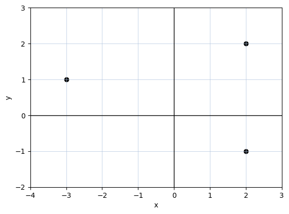
We define three points, two of which lie on a vertical line:
points = np.array([[2, 2], [-3, 1], [2, -1]], dtype=float)

p1, p2, p3 = points
xrange = (-4, 3)
yrange = (-2, 3)

_, ax = plt.subplots()
helpers.prepare_canvas(ax, xrange, yrange)

plt.scatter(points[:, 0], points[:, 1], color='black')

plt.show()
First, we create homoegeneous vector for each point, then, we perfrom cross product between the pairs of interest:
line1 = np.cross(e2h(p1), e2h(p2))
line2 = np.cross(e2h(p1), e2h(p3))
Let’s look what we get as a result:
print(f'line 1: {line1}')
print(f'line 2: {line2}')
line 1: [ 1. -5.  8.]
line 2: [ 3.  0. -6.]
We can also take a look at the normalized vectors:
print(f'line 1: {hnormalize(line1)}')
print(f'line 2: {hnormalize(line2)}')
line 1: [ 0.125 -0.625  1.   ]
line 2: [-0.5 -0.   1. ]
Let’s now visualize the lines to check whether the result is correct:
def plot_line(line_vec, xs, **kwargs):

    # a*x + b*y + c = 0
    assert len(line_vec) == 3
    a, b, c = line_vec

    if b == 0:
        plt.axvline(-c / a, **kwargs)
        return

    slope = -a / b
    intercept = -c / b

    ys = slope * xs + intercept

    plt.plot(xs, ys, **kwargs)
_, ax = plt.subplots()
helpers.prepare_canvas(ax, xrange, yrange)

plt.scatter(points[:, 0], points[:, 1], color='black')

plot_line(line1, np.linspace(*xrange), linestyle='-', color='dodgerblue')
plot_line(line2, np.linspace(*xrange), linestyle='-', color='lawngreen')

plt.show()
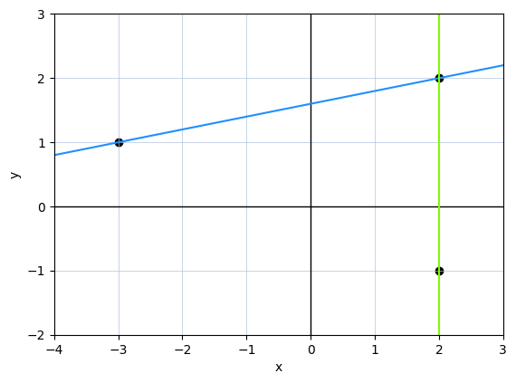
Everything looks correct. How about the dual problem? We see in the plot above that the two lines intesect at the point $[1, 2]^T$. Can we get the same value using the cross-product rule?
p = np.cross(line1, line2)

print('Point at the intersection of the two lines:', h2e(p))
Point at the intersection of the two lines: [2. 2.]
The obtained result is as expected.
To conclude, here are some more in-depth material about homogeneous coordinates and projective geometry:
- “Multiple View Geometry in Computer Vision”, a book by Richard Hartley and Andrew Zisserman
- Explaining Homogeneous Coordinates & Projective Geometry
- Homogeneous Coordinates (part of the course materials on Image Processing and Computer Vision)
- Using Homography for Pose Estimation in OpenCV
- Image Geometric Transformation In Numpy and OpenCV