A homogeneneous transformation is a matrix containing information about rotation and translation. In two dimension, this accounts for an $SO(2)$ rotation matrix (2 x 2) and a translation vector in $\mathbb{R}^2$:

$$ \mathbf{T} = \begin{bmatrix} r_{11} & r_{12} & t_x\cr r_{21} & r_{22} & t_y\cr 0 & 0 & 1 \end{bmatrix} $$

To perform roation and translation of a vector $[x, y]^T$, it is multiplied with $\mathbf{T}$ as a homogeneous vector:

$$ c \begin{bmatrix} x_{new}\cr y_{new}\cr 1 \end{bmatrix} = \begin{bmatrix} r_{11} & r_{12} & t_x\cr r_{21} & r_{22} & t_y\cr 0 & 0 & 1 \end{bmatrix} % \begin{bmatrix} x\cr y\cr 1 \end{bmatrix} $$

The latter expression is equivalent to translation followed by rotation:

$$ \begin{bmatrix} x_{new}\cr y_{new}\cr \end{bmatrix} = \begin{bmatrix} r_{11} & r_{12}\cr r_{21} & r_{22} \end{bmatrix} % \begin{bmatrix} x\cr y \end{bmatrix} + \begin{bmatrix} t_x\cr t_y \end{bmatrix} $$

Using homogeneous transoformation allows not only for performing rotation and translation in one step, but also compounding several transformations. Let’s see this in action with some concrete code examples. As usual, we start with importing the libraries we need.

import numpy as np
from matplotlib import pyplot as plt

np.set_printoptions(formatter={'float_kind': "{: .3f}".format})

First, let’s define a function returing a rotation martix in 2D:

def rotation_matrix(theta):

    c = np.cos(theta)
    s = np.sin(theta)
    
    return np.array([[c, -s], [s, c]])

The next funtion will construct a homogenenous transformation given translation $(t_x, t_y)$ and rotation angle $\theta$:

def create_transform(t_x, t_y, theta):
    
    translation = np.array([t_x, t_y])
    rotation = rotation_matrix(theta)
    
    transform = np.eye(3, dtype=float)
    transform[:2, :2] = rotation
    transform[:2, 2] = translation
    
    return transform

To apply a transfromation, you multiply it with the vector in homogeneous form. The resulting Euclidean vector is obtained by nomalizing the homohenous result (division by the last element):

def apply_transform(transform, x):
    
    x_h = np.ones((x.shape[0] + 1, x.shape[1]), dtype=x.dtype)
    x_h[:-1, :] = x
    
    x_t = np.dot(transform, x_h)
    
    return x_t[:2] / x_t[-1]

Let’s see how a homegenous transformation will look like for translation to $[1, 2]$ and rotation of $\pi/3$ radians:

create_transform(1, 2, np.pi / 3)

array([[ 0.500, -0.866,  1.000],
       [ 0.866,  0.500,  2.000],
       [ 0.000,  0.000,  1.000]])

For the next example, we specify a triangle defined with the following corner points:

corners = np.array([
    [0, -0.5], 
    [2, 0], 
    [0, 0.5]
]).T

We must ensure that each point is represented as a column vector:

corners

array([[ 0.000,  2.000,  0.000],
       [-0.500,  0.000,  0.500]])

Next, we define four poses, i.e. combinations of a translation and a rotation:

poses = np.array([
    [0, 0, 0], # no translation or rotation
    [-3, 0, 0], # move 3 units in negative direction
    [1, 2, np.pi / 3], # move to [1, 2] and rotate by pi/3 (counterclockwise)
    [3, -1, -np.pi / 2], # move to [3, -1] and rotate by pi/2 in the clockwise direction
])

Let’s plot all the poses using Matplotlib. For convenience, we define a helper function to visualize an individual object. Next, we render translated and rotated object, along with the attached coordinate frames (with the original “zero” pose shown in blue).

def viz_object(corners, fill_color, fill_alpha=0.7):
    plt.fill(corners[0, :], corners[1, :], color=fill_color, alpha=fill_alpha)

fig, ax = plt.subplots(figsize=(7, 7))
helpers.create_canvas(xlim=(-5, 5), ylim=(-5, 5))

for i, pose in enumerate(poses):
    
    T = create_transform(*pose)
    transformed = apply_transform(T, corners)
    
    color = 'dodgerblue' if i == 0 else 'lightgray'
    viz_object(transformed, fill_color=color)
    helpers.plot_frame(T)
    
    text_coord = transformed[:, 1]
    plt.text(text_coord[0], text_coord[1], i, fontsize='large')

plt.xlabel('x')
plt.ylabel('y')

plt.show()

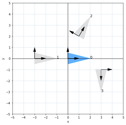
Observe that the visualized object and the coordinate frames correctly correspond the the intended poses:

• (0) no translation or rotation
• (1) move 3 units in negative direction
• (2) move to $[1, 2]$ and rotate by $\pi/3$ (counterclockwise)
• (3) move to $[3, -1]$ and rotate by $\pi/2$ in the clockwise direction

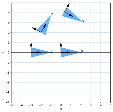
Let’s continue with the same four poses, but now consider the idea of successive transformations: we transfotrm from the original coordinate frame $\lbrace 0 \rbrace$ to frame $\lbrace 1 \rbrace$ using transformation $^0\mathbf{T}_1$, then from $\lbrace 1 \rbrace$ to $\lbrace 2 \rbrace$ using $^1\mathbf{T}_2$, and finally from $\lbrace 2 \rbrace$ to $\lbrace 3 \rbrace$ using $^2\mathbf{T}_3$.

These three successive transformations can be compounded by multiplication from left to right:

$$ ^0\mathbf{T}_3 = (^0\mathbf{T}_1) (^1\mathbf{T}_2) (^2\mathbf{T}_3) $$

This means that given a vector $\mathbf{v}$, we can perform all the three thansforms as follows:

$$ \mathbf{v}_{new} = (^0\mathbf{T}_1) (^1\mathbf{T}_2) (^2\mathbf{T}_3) \mathbf{v} = (^0\mathbf{T}_3) \mathbf{v} $$

Let’s see this in action. We define a function getting an iterable of successive poses, produces a homogeneous transformation for each of them, and multpilies from left to right:

def chain_of_transforms(chain):
    
    result = np.eye(3)
    
    for x, y, theta in chain:
        T = create_transform(x, y, theta)
        result = np.dot(result, T)

    return result

In the next visualization we can trace the successive transformations:

1. From the origin, move 3 units in negative direction
2. From where we are now, move to $[1, 2]$ and rotate by $\pi/3$ (counterclockwise)
3. From where we are now, move to $[3, -1]$ and rotate by $\pi/2$ in the clockwise direction

plt.figure(figsize=(7, 7))
helpers.create_canvas(xlim=(-5, 5), ylim=(-5, 5))

for i, pose in enumerate(poses):

    T = chain_of_transforms(poses[:i+1])
    transformed = apply_transform(T, corners)
    
    viz_object(transformed, fill_color='dodgerblue')
    helpers.plot_frame(T)
    
    text_coord = transformed[:, 1]
    plt.text(text_coord[0], text_coord[1], i, fontsize='large')

plt.xlabel('x')
plt.ylabel('y')

plt.show()

As a final remark, I would like to add about the two interpretations of multiplication $(^A\mathbf{T}_B) \mathbf{v}$:

• Tranform vector $\mathbf{v}$ using translation and rotation encoded in $^A\mathbf{T}_B$ (the interpretation we primarily used in this blog post examples).

• Having a vector $\mathbf{v}$ expressed in the transformed coordinate frame $\lbrace B \rbrace$, obtain its coordinate in the frame $\lbrace A \rbrace$.